SciPy CSGraph

CSGraph stands for Compressed Sparse Graph and focuses on fast graph algorithms based on sparse matrix representations.

Graph Representation

First, let’s understand what a sparse graph is and how it helps with graph representation.

What exactly is a sparse graph?

A graph is simply a collection of nodes with links between them. Graphs can represent almost anything—social networks, where each node is a person connected to its acquaintances; images, where each node is a pixel connected to its neighbors; points in a high-dimensional distribution, where each node is connected to its nearest neighbors; and pretty much anything else you can imagine.

A very effective way to represent graph data is with a sparse matrix: let’s call it G. The matrix G is of size N×N, and G[i, j] gives the value of the connection between node “i” and node “j”. Sparse graphs contain mostly zeros—that is, most nodes have only a few connections. This property holds true in most interesting cases.

The creation of the sparse graph submodule was motivated by several algorithms used in scikit-learn, including the following.

• Isomap – A manifold learning algorithm that finds the shortest paths in a graph.

• Hierarchical Clustering – A clustering algorithm based on minimum spanning trees.

• Lineage Decomposition – A projection algorithm based on the Laplacian of sparse graphs.

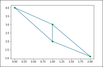
As a concrete example, imagine we want to represent the following undirected graph —

This graph has three nodes, where nodes 0 and 1 are connected by an edge of weight 2, and nodes 0 and 2 are connected by an edge of weight 1. We can construct dense, shielded, and sparse representations as follows, remembering that undirected graphs are represented by a symmetric matrix.

G_dense = np.array([ [0, 2, 1],
                     [2, 0, 0],
                     [1, 0, 0] ])

G_masked = np.ma.masked_values(G_dense, 0)
from scipy.sparse import csr_matrix

G_sparse = csr_matrix(G_dense)
print G_sparse.data

The above program will produce the following output.

array([2, 1, 2, 1])

This is the same graph as before, except that nodes 0 and 2 are connected by a zero-weight edge. In this case, the dense representation above leads to ambiguity—if zero is a meaningful value, how should a non-edge be represented? In this case, a masked or sparse representation must be used to disambiguate.

Let’s consider the following example.

from scipy.sparse.csgraph import csgraph_from_dense
G2_data = np.array
([
   [np.inf, 2, 0],
   [2, np.inf, np.inf],
   [0, np.inf, np.inf]
])
G2_sparse = csgraph_from_dense(G2_data, null_value=np.inf)
print G2_sparse.data

The above program will produce the following output.

array([ 2., 0., 2., 0.])

Word Ladders Using Sparse Graphs

Word Ladders is a game invented by Lewis Carroll in which words are connected by changing one letter at each step. For example –

ape → apt → ait → bit → big → bag → mag → man

Here, we go from “APE” to “MAN” in seven steps, changing one letter each time. The question is – can we find a shorter path between these words using the same rules? This problem can be naturally formulated as a sparse graph problem. Nodes will correspond to individual words, and we will connect words that differ by at most one letter.

Getting a Word List

Of course, first, we must get a valid word list. I’m running a Mac, and Macs have a word dictionary, the location of which is given in the code block below. If you’re using a different architecture, you may need to search a bit to find your system dictionary.

wordlist = open('/usr/share/dict/words').read().split()
print len(wordlist)

The above program will produce the following output.

235886

We’re looking at words of length 3 now, so let’s select only those that are the correct length. We’ll also remove words that begin with a capital letter (proper nouns) or contain non-alphanumeric characters, such as apostrophes and hyphens. Finally, we’ll ensure that all words are lowercase to facilitate comparison later.

word_list = [word for word in word_list if len(word) == 3]
word_list = [word for word in word_list if word[0].islower()]
word_list = [word for word in word_list if word.isalpha()]
word_list = map(str.lower, word_list)
print len(word_list)

The above program will produce the following output.

1135

We now have a list of 1135 valid three-letter words (the exact number may change depending on the specific list used). Each of these words will become a node in our graph, and we will create edges connecting the nodes associated with each pair of words that differ by only one letter.

import numpy as np
word_list = np.asarray(word_list)

word_list.dtype
word_list.sort()

word_bytes = np.ndarray((word_list.size, word_list.itemsize),
   dtype = 'int8',
   buffer = word_list.data)
print word_bytes.shape

The above program will produce the following output.

(1135, 3)

We’ll use the Hamming distance between each point to determine which pairs of words are connected. The Hamming distance measures the proportion of entries between two vectors that are distinct: the Hamming distance between any two words is equal to 1/N1/N, where N is the number of letters that are connected on the word ladder.

from scipy.spatial.distance import pdist, squareform
from scipy.sparse import csr_matrix
hamming_dist = pdist(word_bytes, metric = 'hamming')
graph = csr_matrix(squareform(hamming_dist < 1.5 / word_list.itemsize))

When comparing distances, we do not use equality, as this can be unstable for floating-point values. As long as no two entries in the word list are identical, inequality produces the expected results. Now that our graph is set up, we will use a shortest path search to find a path between any two words in the graph.

i1 = word_list.searchsorted('ape')
i2 = word_list.searchsorted('man')
print word_list[i1],word_list[i2]

The above program will produce the following output.

ape, man

We need to check if these match because if the words are not in the list, we will get an error in the output. Now, all we need is to find the shortest path between these two indices in the graph. We will use Dijkstra‘s algorithm because it allows us to find a path for just one node.

from scipy.sparse.csgraph import dijkstra
distances, predecessors = dijkstra(graph, indices = i1, return_predecessors = True)
print distances[i2]

The above program will produce the following output.

5.0

Thus, we see that the shortest path between “ape” and “man” consists of only five steps. We can use the predecessors returned by the algorithm to reconstruct this path.

path = []
i = i2

while i != i1:
   path.append(word_list[i])
   i = predecessors[i]

path.append(word_list[i1])
print path[::-1]i2]

The above program will produce the following output.

['ape', 'ope', 'opt', 'oat', 'mat', 'man']