SciPy Interpolation

In this chapter, we will discuss the role of interpolation in SciPy.

What is Interpolation

Interpolation is the process of finding a value between two points on a line or curve. To help us remember its meaning, we should think of the first part of the word, “inter,” as meaning “into,” reminding us to look “inside” our original data. Interpolation is a tool useful not only in statistics, but also in science, business, or whenever we need to predict the value between two existing data points.

Let’s create some data and see how to perform this interpolation using the scipy.interpolate package.

import numpy as np
from scipy import interpolate
import matplotlib.pyplot as plt
x = np.linspace(0, 4, 12)
y = np.cos(x**2/3+4)
print x,y

The above program will produce the following output.

(
   array([0., 0.36363636, 0.72727273, 1.09090909, 1.45454545, 1.81818182,
          2.18181818, 2.54545455, 2.90909091, 3.27272727, 3.63636364, 4.]),

   array([-0.65364362, -0.61966189, -0.51077021, -0.31047698, -0.00715476,
           0.37976236, 0.76715099, 0.99239518, 0.85886263, 0.27994201,
-0.52586509, -0.99582185])
)

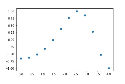
Now, we have two arrays. Assume these two arrays are points in two dimensions in space. Let’s plot them using the following program to see how they look.

plt.plot(x, y,'o')
plt.show()

The above program will produce the following output.

One-Dimensional Interpolation

The interp1d class in scipy.interpolate is a convenient method for creating a function from fixed data points that can be evaluated anywhere within the domain defined by the given data using linear interpolation.

Using the above data, let’s create an interpolation function and plot a new interpolation plot.

f1 = interp1d(x, y, kind = 'linear')

f2 = interp1d(x, y, kind = 'cubic')

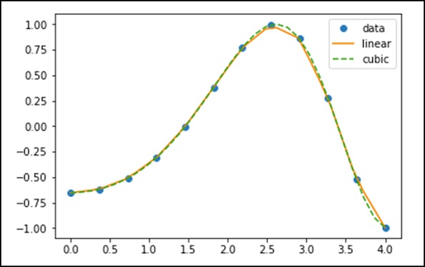
Using the interp1d function, we create two functions, f1 and f2. These functions return y for a given input x. The third variable, kind, represents the type of interpolation technique. Linear, Nearest, Zero, Straight, Quadratic, and Cubic are several interpolation techniques.

Now, let’s create a new input with a larger length to see the noticeable difference in interpolation. We will use the same function on the new data as on the old data.

xnew = np.linspace(0, 4,30)

plt.plot(x, y, ‘o’, xnew, f(xnew), ‘-‘, xnew, f2(xnew), ‘–‘)

plt.legend([‘data’, ‘linear’, ‘cubic’, ‘nearest’], loc = ‘best’)

plt.show()

The above program will produce the following output.

Splines

To draw smooth curves through data points, draftsmen once used flexible thin strips of wood, hard rubber, metal, or plastic called mechanical splines. To use a mechanical spline, points along the curve are judiciously chosen in the design, and the spline is then bent so that it touches each pin.

Clearly, in this construction, the spline interpolates the curve at these pins. It can be used to reproduce the curve on other drawings. The points where the pins are located are called knots. The shape of the curve defined by the spline can be changed by adjusting the position of the knots.

Univariate Spline

A one-dimensional smoothing spline fits a given set of data points. The UnivariateSpline class in scipy.interpolate is a convenient way to create a function based on a fixed set of data points – scipy.interpolate.UnivariateSpline(x, y, w = None, bbox = [None, None], k = 3, s = None, ext = 0, check_finite = False).

Parameters – The following are the parameters for the univariate spline.

• This fits a k-degree spline y = spl(x) to the provided x, y data.

• ‘w’ – Specifies the weight for the spline fit. Must be a positive number. If not present (default), all weights are equal.

• ‘s’ – Specifies the number of knots by specifying a smoothing condition.

• ‘k’ – The degree of the smoothing spline. Must be <= 5. The default is k=3, a cubic spline.

• Ext – Controls the extrapolation mode for elements that are not within the interval defined by the knot sequence.

  • If ext = 0 or ‘extrapolate’, returns the extrapolated value.

  • If ext = 1 or ‘zero’, returns 0.

  • If ext = 2 or ‘raise’, raises a ValueError.

  • If ext = 3 of ‘const’, returns the bounded value.

• check_finite – Whether to check that the input array contains only finite numbers.

Let’s consider the following example.

import matplotlib.pyplot as plt
from scipy.interpolate import UnivariateSpline
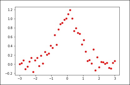
x = np.linspace(-3, 3, 50)
y = np.exp(-x**2) + 0.1 * np.random.randn(50)
plt.plot(x, y, 'ro', ms = 5)
plt.show()

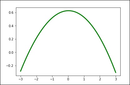
Using the default values for the smoothing parameters.

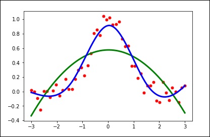
spl = UnivariateSpline(x, y)
xs = np.linspace(-3, 3, 1000)
plt.plot(xs, spl(xs), 'g', lw = 3)
plt.show()

Manually change the amount of smoothing.

spl.set_smoothing_factor(0.5)
plt.plot(xs, spl(xs), 'b', lw = 3)
plt.show()